In this post, we will build a Convolutional Neural Network (CNNs), but we will understand it through images. CNNs are really powerful, and there is a huge body of research that have used CNNs for a variety of tasks. CNNs have become widely popular in text classification systems. CNNs help in reduction in computation by exploiting local correlation of the input data.
A variant of this work essentially describes the approach I took to create a conversational agent as part of my thesis which involved intent classification for a virtual patient training system. 1, 2.
This post relies on a lot of fantastic work that has already been done on convolutions in the text, and here is a list of papers that delve into the details of most of the content I have described here.
- Natural Language Processing (almost) from Scratch
- Character-level Convolutional Networks for Text Classification
- Convolutional Neural Networks for Sentence Classification
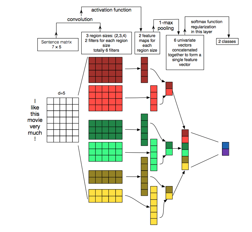
Let’s start with inputs:
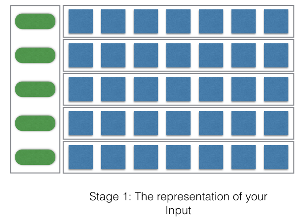
So the green boxes represent the words or the characters depending on your approach. If you are using character based convolutional neural network then it is characters whereas if you are using words as a unit then it is the word based convolution. And the corresponding blue rows represent the representation of the words or the characters. In the case of character based convolutions, since the number of characters was around 70, including punctuations, numbers, and alphabets, this is generally the one-hot representation. In the case of words, the blue boxes generally represent dense vectors. These dense vectors can be pre-trained word embeddings or word vectors trained during training. See my previous blog post about word embeddings here.
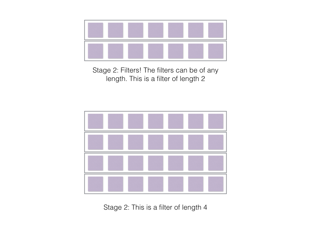
Now as you can see, filters (also known as kernels) can be of any length. Here the length refers to the number of rows of the filter. In the case of images, the width and length of the kernel can be any size. But the width of the kernel in case of character and word representations is the dimension of the entire word embedding or the entire character representation. Thus the only dimension that matters in the case of convolutions in NLP tasks, is the length of the filter or the size of the filter.
Now the filters need to convolve with the input and produce the output. Convolve is a fancy term for multiplication with corresponding cells and adding up the sum. This part is slightly tricky to understand and varies based on things like stride (How much the filter moves every stage?) and the length of the filter. The output of the convolution operation is directly dependent on these two aspects. This will become clearer in the following image.
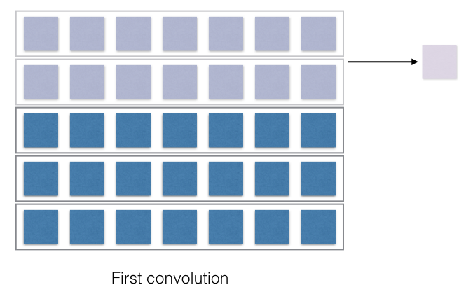
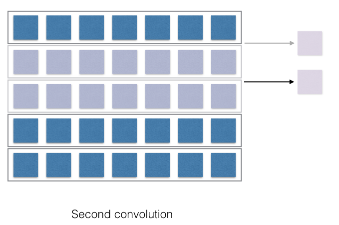
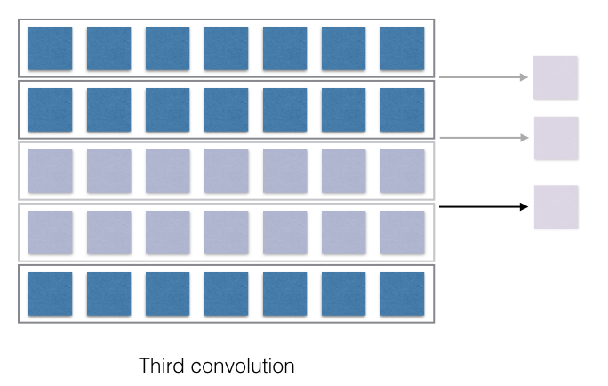
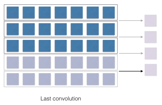
Now, this is where all the interesting bit happens! The convolution is just the multiplication of the weights in the filters and the corresponding representation of the words or characters. Each of the output of the multiplication is then just summed up and it produces one output, shown with the arrow. Thus if the filter would have moved with a stride of 2, then the number of filter outputs would have been different. If the filter length was different, the convolved output would be different. Convince yourself that the filter of the length 4, when convolved, will just produce 2 outputs.
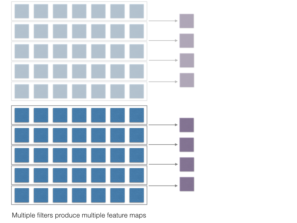
Like multiple filter lengths, there can be multiple filters of the same length. So there can be a 100 filters of length 2, a hundred filters of length 4 and so on.
Each of these will then produce multiple outputs!
The final stage comprises of max pooling then concatenation and softmax regularization.
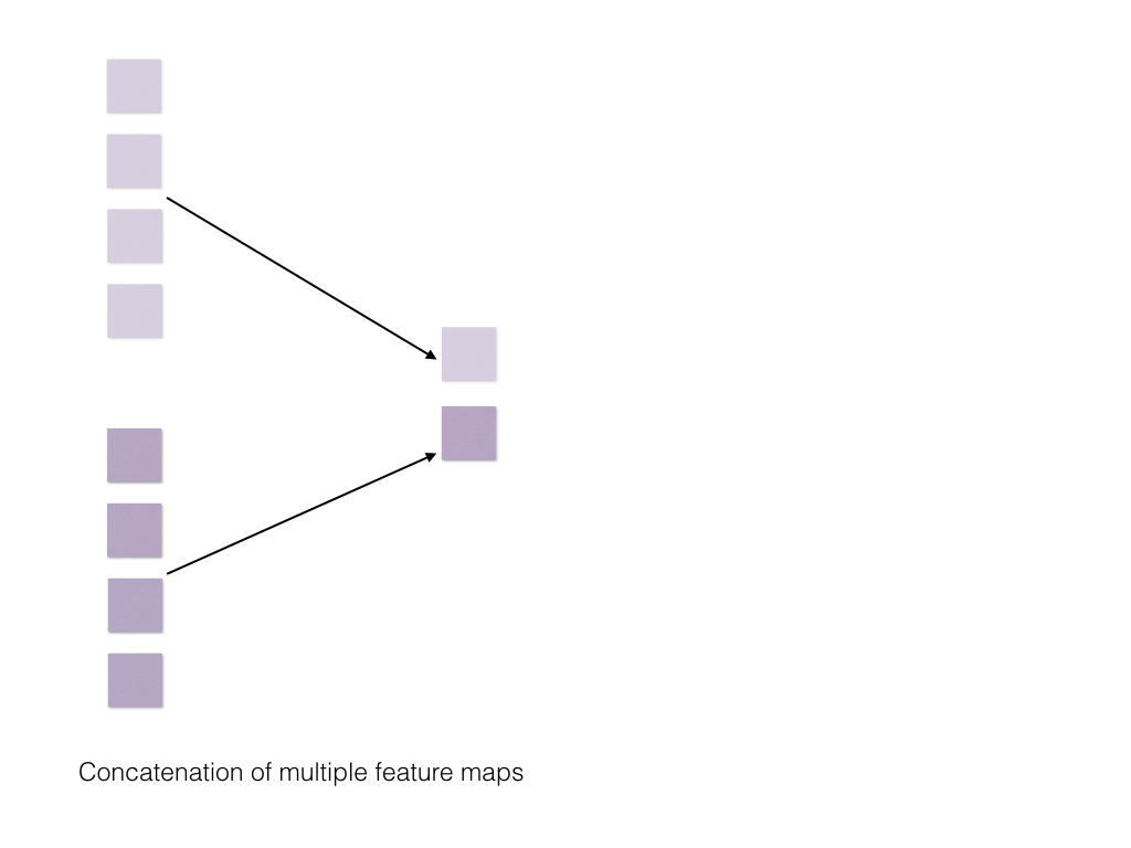
Aha! And that is it! The entire process was very nicely illustrated by Zhang et al, in the paper “A Sensitivity Analysis of (and Practitioners’ Guide to) Convolutional Neural Networks for Sentence Classification”, for words. The above is just replicating the same for characters and how it would appear at every step!
Let’s now dive into the code and explore these features in depth!
Understanding convolutions through code will make the process of understanding CNN really easy and can thus be used for a variety of other tasks.
The task we are trying to accomplish here is to classify text. Specifically, the input to the convolutional network can be words or characters like we discussed before. Here, from the sequence of words, in a sentence or from the sequence of characters in a sentence we would want to classify the category of the sentence, like positive or negative and so on.
This post assumes familiarity with Keras, but that may not be necessary if you just want an overview of the architectures.
The papers we mentioned above, are the ones we will touch upon in this post.
I will use the imdb data for the text classification part of the work instead of the dataset I used for my thesis. The idea and implementation, however, is very similar.
So the data we will be exploring is the imdb sentiment analysis data, that can be found in the UCI Machine Learning Repository here
import pandas as pd
import re
import tensorflow as tf
import numpy as np
from keras.utils.np_utils import to_categorical
Using TensorFlow backend.
data = pd.read_csv("sentiment labelled sentences/imdb_labelled.txt", delimiter='\t', header=None, quoting=3, names=['review','label'])
data = pd.read_csv("sentiment labelled sentences/yelp_labelled.txt", delimiter='\t', header=None, names=['review','label'], encoding='utf-8')
data
| review | label | |
|---|---|---|
| 0 | Wow... Loved this place. | 1 |
| 1 | Crust is not good. | 0 |
| 2 | Not tasty and the texture was just nasty. | 0 |
| 3 | Stopped by during the late May bank holiday of... | 1 |
| 4 | The selection on the menu was great and so wer... | 1 |
| 5 | Now I am getting angry and I want my damn pho. | 0 |
| 6 | Honeslty it didn't taste THAT fresh.) | 0 |
| 7 | The potatoes were like rubber and you could te... | 0 |
| 8 | The fries were great too. | 1 |
| 9 | A great touch. | 1 |
| 10 | Service was very prompt. | 1 |
| 11 | Would not go back. | 0 |
| 12 | The cashier had no care what so ever on what I... | 0 |
| 13 | I tried the Cape Cod ravoli, chicken,with cran... | 1 |
| 14 | I was disgusted because I was pretty sure that... | 0 |
| 15 | I was shocked because no signs indicate cash o... | 0 |
| 16 | Highly recommended. | 1 |
| 17 | Waitress was a little slow in service. | 0 |
| 18 | This place is not worth your time, let alone V... | 0 |
| 19 | did not like at all. | 0 |
| 20 | The Burrittos Blah! | 0 |
| 21 | The food, amazing. | 1 |
| 22 | Service is also cute. | 1 |
| 23 | I could care less... The interior is just beau... | 1 |
| 24 | So they performed. | 1 |
| 25 | That's right....the red velvet cake.....ohhh t... | 1 |
| 26 | - They never brought a salad we asked for. | 0 |
| 27 | This hole in the wall has great Mexican street... | 1 |
| 28 | Took an hour to get our food only 4 tables in ... | 0 |
| 29 | The worst was the salmon sashimi. | 0 |
| ... | ... | ... |
| 970 | I immediately said I wanted to talk to the man... | 0 |
| 971 | The ambiance isn't much better. | 0 |
| 972 | Unfortunately, it only set us up for disapppoi... | 0 |
| 973 | The food wasn't good. | 0 |
| 974 | Your servers suck, wait, correction, our serve... | 0 |
| 975 | What happened next was pretty....off putting. | 0 |
| 976 | too bad cause I know it's family owned, I real... | 0 |
| 977 | Overpriced for what you are getting. | 0 |
| 978 | I vomited in the bathroom mid lunch. | 0 |
| 979 | I kept looking at the time and it had soon bec... | 0 |
| 980 | I have been to very few places to eat that und... | 0 |
| 981 | We started with the tuna sashimi which was bro... | 0 |
| 982 | Food was below average. | 0 |
| 983 | It sure does beat the nachos at the movies but... | 0 |
| 984 | All in all, Ha Long Bay was a bit of a flop. | 0 |
| 985 | The problem I have is that they charge $11.99 ... | 0 |
| 986 | Shrimp- When I unwrapped it (I live only 1/2 a... | 0 |
| 987 | It lacked flavor, seemed undercooked, and dry. | 0 |
| 988 | It really is impressive that the place hasn't ... | 0 |
| 989 | I would avoid this place if you are staying in... | 0 |
| 990 | The refried beans that came with my meal were ... | 0 |
| 991 | Spend your money and time some place else. | 0 |
| 992 | A lady at the table next to us found a live gr... | 0 |
| 993 | the presentation of the food was awful. | 0 |
| 994 | I can't tell you how disappointed I was. | 0 |
| 995 | I think food should have flavor and texture an... | 0 |
| 996 | Appetite instantly gone. | 0 |
| 997 | Overall I was not impressed and would not go b... | 0 |
| 998 | The whole experience was underwhelming, and I ... | 0 |
| 999 | Then, as if I hadn't wasted enough of my life ... | 0 |
1000 rows × 2 columns
Character based CNN
docs = []
sentences = []
sentiments = []

for sentences, sentiment in zip(data.review, data.label):
    sentences_cleaned = [sent.lower() for sent in sentences]
    docs.append(sentences_cleaned)
    sentiments.append(sentiment)
len(docs), len(sentiments)
(1000, 1000)
Now that we have documents of length 1000, and sentiments of length 1000, let’s do the NLP part.
maxlen = 1024 # In the original paper for character level convolutions, Zhang et al. used
# a maxlen of 1014. Just using 1024, because for the sake of consitency, of comparison
# with the next model. Also, the number 1014 kinda bothered me. 1024 makes me feel a lot better.
nb_filter = 256
dense_outputs = 1024
filter_kernels = [7, 7, 3, 3, 3, 3]
n_out = 2
batch_size = 80
nb_epoch = 10
txt = ''
for doc in docs:
    for s in doc:
        txt += s
chars = set(txt)
vocab_size = len(chars)
print('total chars:', len(chars))
char_indices = dict((c, i) for i, c in enumerate(chars))
indices_char = dict((i, c) for i, c in enumerate(chars))
('total chars:', 56)
Here we have a total of 57 characters. In the original paper, the number of characters was 70, which included 26 English letters, 10 digits, 33 other characters and the new line character. The non-space characters are:
abcdefghijklmnopqrstuvwxyz0123456789
-,;.!?:’’’/|_@#$%ˆ&*˜‘+-=<>()[]{}
Before the convolutions, we need the data to the neural network to be of a particular format.
The format is as follows:
Number_of_Reviews X maxlen X Vocab_Size
from keras.preprocessing.sequence import pad_sequences
def vectorize_sentences(data, char_indices):
    X = []
    for sentences in data:
        x = [char_indices[w] for w in sentences]
        x2 = np.eye(len(char_indices))[x]
        X.append(x2)
    return (pad_sequences(X, maxlen=maxlen))
train_data = vectorize_sentences(docs,char_indices)
train_data.shape
y_train = to_categorical(sentiments)
Now we have the data in the right format! Number_of_Reviews X maxlen X Vocab_Size
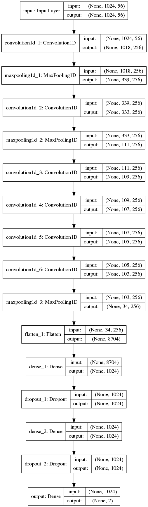
Now the model is fairly simple. Here are the details:
from keras.models import Model
from keras.layers import Input, Dense, Dropout, Flatten
from keras.layers.convolutional import Convolution1D, MaxPooling1D

inputs = Input(shape=(maxlen, vocab_size), name='input', dtype='float32')

conv = Convolution1D(nb_filter=nb_filter, filter_length=filter_kernels[0],
                     border_mode='valid', activation='relu',
                     input_shape=(maxlen, vocab_size))(inputs)
conv = MaxPooling1D(pool_length=3)(conv)

conv1 = Convolution1D(nb_filter=nb_filter, filter_length=filter_kernels[1],
                      border_mode='valid', activation='relu')(conv)
conv1 = MaxPooling1D(pool_length=3)(conv1)

conv2 = Convolution1D(nb_filter=nb_filter, filter_length=filter_kernels[2],
                      border_mode='valid', activation='relu')(conv1)

conv3 = Convolution1D(nb_filter=nb_filter, filter_length=filter_kernels[3],
                      border_mode='valid', activation='relu')(conv2)

conv4 = Convolution1D(nb_filter=nb_filter, filter_length=filter_kernels[4],
                      border_mode='valid', activation='relu')(conv3)

conv5 = Convolution1D(nb_filter=nb_filter, filter_length=filter_kernels[5],
                      border_mode='valid', activation='relu')(conv4)
conv5 = MaxPooling1D(pool_length=3)(conv5)
conv5 = Flatten()(conv5)

z = Dropout(0.5)(Dense(dense_outputs, activation='relu')(conv5))
z = Dropout(0.5)(Dense(dense_outputs, activation='relu')(z))

pred = Dense(n_out, activation='softmax', name='output')(z)

model = Model(input=inputs, output=pred)

model.compile(loss='categorical_crossentropy', optimizer='rmsprop',
              metrics=['accuracy'])

# model.fit(train_data, y_train, batch_size=32,
#            nb_epoch=120, validation_split=0.2, verbose=False)


from keras.utils.visualize_util import model_to_dot
from IPython.display import Image

Image(model_to_dot(model, show_shapes=True).create(prog='dot', format='png'))
Word based CNN
The next part, we will use convolutions on words. Since convolutions on words also have produced really good results.
Now the input data needs to be in the form:
Number_of_reviews X maxlen
So let’s process the data in that format. Here we will use a variation of Yoon Kim’s paper. Now the imdb data is really small, for these to be very effective. But hopefully, this will be sufficient for you to do experiments with your own data sets.
For tokenization, there is a fantastic NLP library, Spacy that has become popular recently, and we will use that. Tokenization the right way is a very important task and can drastically affect the result. For instance, if you just decide to tokenize based on space then the word ‘did’ will have two representations in ‘did!’ and ‘did’. You can even define custom rules for tokenization based on your dataset. Spacy has a really good example of that here. Since the IMDB dataset is a relatively clean one, we will just use the default tokenizer that spacy gives us. Feel free to experiment with the variety of options Spacy provides.
Examples: ‘did!’ and ‘did’
data = pd.read_csv("sentiment labelled sentences/yelp_labelled.txt",
                   delimiter='\t', header=None, names=['review','label'],encoding='utf-8')
# z = list(nlp.pipe(data['review'], n_threads=20, batch_size=20000))

from __future__ import unicode_literals
from spacy.en import English
from collections import Counter

raw_text = 'Hello, world. Here are two sentences.'
nlp = English()
def tokenizeSentences(sent):
    doc = nlp(sent)
    sentences = [sent.string.strip() for sent in doc]
    return sentences
Xs = []
for texts in data['review']:
    Xs.append(tokenizeSentences(texts))
Xs
[[u'Wow', u'...', u'Loved', u'this', u'place', u'.'],
 [u'Crust', u'is', u'not', u'good', u'.'],
 [u'Not',
  u'tasty',
  u'and',
  u'the',
  u'texture',
  u'was',
  u'just',
  u'nasty',
  u'.']]
vocab = sorted(reduce(lambda x, y: x | y, (set(words) for words in Xs)))
len(vocab)
2349
At this stage, you can go ahead with this vocab, but ideally, we would want to get rid of the very infrequent words. So cases where the tokenizer failed, or the emoticons and so on. This is because if someone used the word ‘amaaazzziiinggg’ or ‘Wooooooow’ to describe the movie we do not want to create two different tokens for the word ‘amazing’. Also, you can define custom rules in Spacy to take these into account. Secondly, another option that is often followed in information retrieval approaches is to get rid of the most frequent words. This is because words like ‘the’, ‘an’ and so on occur very frequently and do not add to the meaning. We will ignore this part of the IMDB dataset since it is already really small but the following code snippet will help you get rid of the most frequent and the least frequent words in case you desire so.
So let’s build a function to get words that have at least appeared more than once in our vocab. The reason for doing this, instead of selecting the most frequent 500 words, is that there will be a lot of words that get eliminated arbitrarily as soon as we reach the 500-word limit. (A lot of words have very similar counts!)
import operator

def word_freq(Xs, num):
    all_words = [words.lower() for sentences in Xs for words in sentences]
    sorted_vocab = sorted(dict(Counter(all_words)).items(), key=operator.itemgetter(1))
    final_vocab = [k for k,v in sorted_vocab if v>num]
    word_idx = dict((c, i + 1) for i, c in enumerate(final_vocab))
    return final_vocab, word_idx
final_vocab, word_idx = word_freq(Xs,2)
vocab_len = len(final_vocab) # Finally we have 598 words!
Here is something I do often during text processing. The vectorize function will vectorize the words we have. Now there are three possible scenarios that can occur. Because we didn’t specifically lower case all the words: the word is in the dictionary and we found it the lower case word is in the dictionary and we found it the word is not in the dictionary
def vectorize_sentences(data, word_idx, final_vocab, maxlen=40):
    X = []
    paddingIdx = len(final_vocab)+2
    for sentences in data:
        x=[]
        for word in sentences:
            if word in final_vocab:
                x.append(word_idx[word])
            elif word.lower() in final_vocab:
                x.append(word_idx[word.lower()])
            else:
                x.append(paddingIdx)
        X.append(x)
    return (pad_sequences(X, maxlen=maxlen))
train_data = vectorize_sentences(Xs, word_idx, final_vocab)
train_data.shape
(1000, 40)
The following convolution architecture is very similar to the one proposed by Kim et al., except here we are not using pre-trained word embeddings. The addition of pre-trained word embeddings should be fairly simple. Here is a nice example, on the keras blog.
https://blog.keras.io/
from keras.layers.core import Activation, Flatten, Dropout, Dense, Merge
from keras.layers import Convolution1D
from keras.layers.pooling import MaxPooling1D
from keras.models import Sequential
from keras.layers.embeddings import Embedding
from keras.optimizers import Adam, rmsprop


n_in = 40
EMBEDDING_DIM=100
filter_sizes = (2,4,5,8)
dropout_prob = [0.4,0.5]

graph_in = Input(shape=(n_in, EMBEDDING_DIM))
convs = []
avgs = []
for fsz in filter_sizes:
    conv = Convolution1D(nb_filter=32,
                         filter_length=fsz,
                         border_mode='valid',
                         activation='relu',
                         subsample_length=1)(graph_in)
    pool = MaxPooling1D(pool_length=n_in-fsz+1)(conv)
    flattenMax = Flatten()(pool)
    convs.append(flattenMax)

if len(filter_sizes)>1:
    out = Merge(mode='concat')(convs)
else:
    out = convs[0]

graph = Model(input=graph_in, output=out, name="graphModel")


model = Sequential()
model.add(Embedding(input_dim=vocab_len, #size of vocabulary
                 output_dim = EMBEDDING_DIM,
                 input_length = n_in,
                 trainable=True))
model.add(Dropout(dropout_prob[0]))
model.add(graph)
model.add(Dense(128))
model.add(Dropout(dropout_prob[1]))
model.add(Activation('relu'))
model.add(Dense(2))
model.add(Activation('sigmoid'))

number_of_epochs = 50
# adam = Adam(clipnorm=.1)
model.compile(loss='categorical_crossentropy',
              optimizer='adam',
              metrics=['acc'])
train_data.shape, y_train.shape
((1000, 40), (1000, 2))
model.fit(train_data, y_train, batch_size=32,
           nb_epoch=10, validation_split=0.2, verbose=True)
Train on 800 samples, validate on 200 samples
Epoch 1/10
800/800 [==============================] - 0s - loss: 0.0542 - acc: 0.9838 - val_loss: 0.5125 - val_acc: 0.7850
Epoch 2/10
800/800 [==============================] - 0s - loss: 0.0305 - acc: 0.9950 - val_loss: 0.7075 - val_acc: 0.7700
Epoch 3/10
800/800 [==============================] - 0s - loss: 0.0288 - acc: 0.9937 - val_loss: 0.7525 - val_acc: 0.7700
Epoch 4/10
800/800 [==============================] - 0s - loss: 0.0204 - acc: 0.9950 - val_loss: 0.8603 - val_acc: 0.7600
Epoch 5/10
800/800 [==============================] - 0s - loss: 0.0116 - acc: 0.9975 - val_loss: 0.6404 - val_acc: 0.7950
Epoch 6/10
800/800 [==============================] - 0s - loss: 0.0242 - acc: 0.9937 - val_loss: 0.7380 - val_acc: 0.7800
Epoch 7/10
800/800 [==============================] - 0s - loss: 0.0141 - acc: 0.9975 - val_loss: 0.5975 - val_acc: 0.8050
Epoch 8/10
800/800 [==============================] - 0s - loss: 0.0123 - acc: 0.9975 - val_loss: 0.8370 - val_acc: 0.7700
Epoch 9/10
800/800 [==============================] - 0s - loss: 0.0093 - acc: 0.9988 - val_loss: 0.7746 - val_acc: 0.7800
Epoch 10/10
800/800 [==============================] - 0s - loss: 0.0102 - acc: 0.9962 - val_loss: 0.7894 - val_acc: 0.7900


<keras.callbacks.History at 0x7f071234ea50>